Indexing (Part 2) and Views
March 4, 2021
Garcia-Molina/Ullman/Widom: Papers and Ch. 8.1-8.2
Today
- How do we keep a list sorted under updates?
- Can we "compress" an ISAM index?
- Other ways to accelerate queries.
Access Paths
Reads Want: Nice sorted, compact list.
Writes Want: Random order.
What happens if we optimize for reads
(and even do away with pages)
Each insert requires $O(N)$ write IOs.
"Write Amplification"
How can we reduce Write Amplification?
Idea: Buffer writes
Pro: With a $\mathcal B$ element buffer, $O(\frac{N}{\mathcal B})$ write amplification (amortized)
Con: Every read now needs to go to two places
Con: $O(\frac{N}{\mathcal B})$ is still linear
Idea: Don't merge!
Pro: No write amplification!
Con: Every read now needs to go to $O(\frac{N}{B})$ places on disk (Read Amplification)
Idea: Combine the two?
Log-Structured Merge (LSM) Trees
- Buffer contains $\mathcal B$ records
- Level 1 contains $\mathcal B$ records
- Level 2 contains $2\mathcal B$ records
- Level 3 contains $4\mathcal B$ records
In general, level $i$ contains $2^{i-1} \mathcal B$ records.
When writing to a full level, merge and write to next level instead.
Basic LSM Trees
Write Amplification: Every record copied $O(\log N)$ times
Read Amplification: At most $O(\log N)$ levels
LSM Trees in Practice
- LevelDB/RocksDB
- Apache Cassandra
- Google Bigtable
- HBase
Other design choices
- Fanout
- Instead of doubling the size of each level, have each level grow by a factor of $K$. Level $i$ is merged into level $i+1$ when its size grows above $K^{i-1}$.
- "Tiered" (instead of "Leveled")
- Store each level as $K$ sorted runs instead of proactively merging them. Merge the runs together when escalating them to the next level.
CDF-Based Indexing
"The Case for Learned Index Structures"
by Kraska, Beutel, Chi, Dean, Polyzotis
Cumulative Distribution Function (CDF)
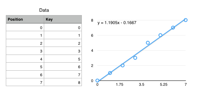
$f(key) \mapsto position$
(not exactly true, but close enough for today)
Using CDFs to find records
- Ideal: $f(k) = position$
- $f$ encodes the exact location of a record
- Ok: $f(k) \approx position$
$\left|f(k) - position\right| < \epsilon$ - $f$ gets you to within $\epsilon$ of the key
- Only need local search on one (or so) leaf pages.
Simplified Use Case: Static data with "infinite" prep time.
How to define $f$?
- Linear ($f(k) = a\cdot k + b$)
- Polynomial ($f(k) = a\cdot k + b \cdot k^2 + \ldots$)
- Neural Network ($f(k) = $
 )
)
We have infinite prep time, so fit a (tiny) neural network to the CDF.
Neural Networks
- Extremely Generalized Regression
- Essentially a really really really complex, fittable function with a lot of parameters.
- Captures Nonlinearities
- Most regressions can't handle discontinuous functions, which many key spaces have.
- No Branching
ifstatements are really expensive on modern processors.- (Compare to B+Trees with $\log_2 N$ if statements)
Summary
- Tree Indexes
- $O(\log N)$ access, supports range queries, easy size changes.
- Hash Indexes
- $O(1)$ access, doesn't change size efficiently, only equality tests.
- LSM Trees
- $O(K\log(\frac{N}{B}))$ access. Good for update-unfriendly filesystems.
- CDF Indexes
- $O(1)$ access, supports range queries, static data only.
Views
      SELECT partkey
      FROM lineitem l, orders o
      WHERE l.orderkey = o.orderkey
      AND o.orderdate >= DATE(NOW() - '1 Month')
      ORDER BY shipdate DESC LIMIT 10;
      SELECT suppkey, COUNT(*)
      FROM lineitem l, orders o
      WHERE l.orderkey = o.orderkey
      AND o.orderdate >= DATE(NOW() - '1 Month')
      GROUP BY suppkey;
      SELECT partkey, COUNT(*)
      FROM lineitem l, orders o
      WHERE l.orderkey = o.orderkey
      AND o.orderdate > DATE(NOW() - '1 Month')
      GROUP BY partkey;
All of these views share the same business logic!
Started as a convenience
      CREATE VIEW salesSinceLastMonth AS
        SELECT l.*
        FROM lineitem l, orders o
        WHERE l.orderkey = o.orderkey
        AND o.orderdate > DATE(NOW() - '1 Month')
      SELECT partkey FROM salesSinceLastMonth
      ORDER BY shipdate DESC LIMIT 10;
      SELECT suppkey, COUNT(*)
      FROM salesSinceLastMonth
      GROUP BY suppkey;
      SELECT partkey, COUNT(*)
      FROM salesSinceLastMonth
      GROUP BY partkey;
But also useful for performance
      CREATE MATERIALIZED VIEW salesSinceLastMonth AS
        SELECT l.*
        FROM lineitem l, orders o
        WHERE l.orderkey = o.orderkey
        AND o.orderdate > DATE(NOW() - '1 Month')
Materializing the view, or pre-computing and saving the view lets us answer all of the queries on the view faster!
What if the query doesn't use the view?
      SELECT l.partkey
      FROM lineitem l, orders o
      WHERE l.orderkey = o.orderkey
      AND o.orderdate > DATE(’2015-03-31’)
      ORDER BY l.shipdate DESC
      LIMIT 10;
Can we detect that a query could be answered with a view?
(sometimes)
| View Query | User Query | |
|---|---|---|
SELECT $L_v$FROM $R_v$WHERE $C_v$
|
SELECT $L_q$FROM $R_q$WHERE $C_q$
|
When are we allowed to rewrite this table?
| View Query | User Query | |
|---|---|---|
SELECT $L_v$FROM $R_v$WHERE $C_v$
|
SELECT $L_q$FROM $R_q$WHERE $C_q$
|
- $R_V \subseteq R_Q$
- All relations in the view are part of the query join
- $C_Q = C_V \wedge C'$
- The view condition is 'weaker' than the query condition
- $attrs(C') \cap attrs(R_V) \subseteq L_V$ $L_Q \cap attrs(R_V) \subseteq L_V$
- The view doesn't project away needed attributes
| View Query | User Query | |
|---|---|---|
SELECT $L_v$FROM $R_v$WHERE $C_v$
|
SELECT $L_q$FROM $R_q$WHERE $C_q$
|
SELECT $L_Q$FROM $(R_Q - R_V)$, viewWHERE $C_Q$
Summary
- For each relation, identify candidate indexes
- For each join, identify candidate indexes
- Identify candidate views
- Identify available join, aggregate, sort algorithms
Enumerate all possible plans
... then how do you pick? (more soon)